🏷️ How to label your data and fine-tune a 🤗 sentiment classifier
This tutorial will show you how to fine-tune a sentiment classifier for your own domain, starting with no labeled data.
Most online tutorials about fine-tuning models assume you already have a training dataset. You’ll find many tutorials for fine-tuning a pre-trained model with widely-used datasets, such as IMDB for sentiment analysis.
However, very often what you want is to fine-tune a model for your use case. It’s well-known that NLP model performance degrades with “out-of-domain” data. For example, a sentiment classifier pre-trained on movie reviews (e.g., IMDB) will not perform very well with customer requests.
In this tutorial, we’ll build a sentiment classifier for user requests in the banking domain as follows:
🏁 Start with the most popular sentiment classifier on the Hugging Face Hub (2.3 million monthly downloads as of July 2021) which has been fine-tuned on the SST2 sentiment dataset.
🏷️ Label a training dataset with banking user requests starting with the pre-trained sentiment classifier predictions.
⚙️ Fine-tune the pre-trained classifier with your training dataset.
🏷️ Label more data by correcting the predictions of the fine-tuned model.
⚙️ Fine-tune the pre-trained classifier with the extended training dataset.
This is an overview of the workflow we’ll be following:

Let’s get started!
Setup Rubrix
If you are new to Rubrix, visit and star Rubrix for updates: ⭐ Github repository
If you have not installed and launched Rubrix, check the Setup and Installation guide.
Once installed, you only need to import Rubrix:
[1]:
import rubrix as rb
Install tutorial dependencies
In this tutorial, we’ll use the transformers and datasets libraries.
[ ]:
%pip install transformers -qqq
%pip install datasets -qqq
Preliminaries
For building our fine-tuned classifier we’ll be using two main resources, both available in the 🤗 Hub :
A dataset in the banking domain:
banking77A pre-trained sentiment classifier:
distilbert-base-uncased-finetuned-sst-2-english
Dataset: Banking 77
This dataset contains online banking user queries annotated with their corresponding intents.
In our case, we’ll label the sentiment of these queries, which might be useful for digital assistants and customer service analytics.
Let’s load the dataset directly from the hub:
[ ]:
from datasets import load_dataset

banking_ds = load_dataset("banking77")
For this tutoral, let’s split the dataset into two 50% splits. We’ll start with the to_label1 split for data exploration and annotation and keep to_label2 for further iterations.
[ ]:
to_label1, to_label2 = banking_ds['train'].train_test_split(test_size=0.5, seed=42).values()
Model: sentiment distilbert fine-tuned on sst-2
As of July 2021, the distilbert-base-uncased-finetuned-sst-2-english is the most popular text-classification model in the Hugging Face Hub.
This model is a distilbert model fine-tuned on the highly popular sentiment classification benchmark SST-2 (Stanford Sentiment Treebank).
As we will see later, this is a general-purpose sentiment classifier, which will need further fine-tuning for specific use cases and styles of text. In our case, we’ll explore its quality on banking user queries and build a training set for adapting it to this domain.
[6]:
from transformers import pipeline

sentiment_classifier = pipeline(
    model="distilbert-base-uncased-finetuned-sst-2-english",
    task="sentiment-analysis",
    return_all_scores=True,
)
Now let’s test this pipeline with an example of our dataset:
[15]:
to_label1[3]['text'], sentiment_classifier(to_label1[3]['text'])
[15]:
('I just have one additional card from the USA. Do you support that?',
 [[{'label': 'NEGATIVE', 'score': 0.5619744062423706},
   {'label': 'POSITIVE', 'score': 0.43802565336227417}]])
The model assigns more probability to the NEGATIVE class. Following our annotation policy (read more below), we’ll label examples like this as POSITIVE as they are general questions, not related to issues or problems with the banking application. The ultimate goal will be to fine-tune the model to predict POSITIVE for these cases.
A note on sentiment analysis and data annotation
Sentiment analysis is one of the most subjective tasks in NLP. What we understand by sentiment will vary from one application to another and depend on the business objectives of the project. Also, sentiment can be modeled in different ways, leading to different labeling schemes. For example, sentiment can be modeled as real value (going from -1 to 1, from 0 to 1.0, etc.) or with 2 or more labels (including different degrees such as positive, negative, neutral, etc.)
For this tutorial, we’ll use the original labeling scheme defined by the pre-trained model which is composed of two labels: POSITIVE and NEGATIVE. We could have added the NEUTRAL label, but let’s keep it simple.
Another important issue when approaching a data annotaion project are the annotation guidelines, which explain how to assign the labels to specific examples. As we’ll see later, the messages we’ll be labeling are mostly questions with a neutral sentiment, which we’ll label with the POSITIVE label, and some other are negative questions which we’ll label with the NEGATIVE label. Later on, we’ll show some examples of each label.
1. Run the pre-trained model over the dataset and log the predictions
As a first step, let’s use the pre-trained model for predicting over our raw dataset. For this will use the handy dataset.map method from the datasets library.

Predict
[16]:
def predict(examples):
    return {"predictions": sentiment_classifier(examples['text'], truncation=True)}
[ ]:
to_label1 = to_label1.map(predict, batched=True, batch_size=4)
Log
The following code builds a list of Rubrix records with the predictions and logs them into a Rubrix Dataset. We’ll use this dataset to explore and label our first training set.
[18]:
records = []
for example in to_label1.shuffle():
    record = rb.TextClassificationRecord(
        inputs=example["text"],
        metadata={'category': example['label']}, # log the intents for exploration of specific intents
        prediction=[(pred['label'], pred['score']) for pred in example['predictions']],
        prediction_agent="distilbert-base-uncased-finetuned-sst-2-english"
    )
    records.append(record)
[ ]:
rb.log(name='labeling_with_pretrained', records=records)
2. Explore and label data with the pretrained model
In this step, we’ll start by exploring how the pre-trained model is performing with our dataset.
At first sight:
The pre-trained sentiment classifier tends to label most of the examples as
NEGATIVE(4.835 of 5.001 records). You can see this yourself using thePredictions / Predicted as:filterUsing this filter and filtering by predicted as
POSITIVE, we see that examples like “I didn’t withdraw the amount of cash that is showing up in the app.” are not predicted as expected (according to our basic “annotation policy” described in the preliminaries).
Taking into account this analysis, we can start labeling our data.

Rubrix provides you with a search-driven UI to annotated data, using free-text search, search filters and the Elasticsearch query DSL for advanced queries. This is most useful for sparse datasets, tasks with a high number of labels or unbalanced classes. In the standard case, we recommend you to follow the workflow below:
Start labeling examples sequentially, without using search features. This way you’ll annotate a fraction of your data which will be aligned with the dataset distribution.
Once you have a sense of the data, you can start using filters and search features to annotate examples with specific labels. In our case, we’ll label examples predicted as
POSITIVEby our pre-trained model, and then a few examples predicted asNEGATIVE.
Labeling random examples

Labeling POSITIVE examples

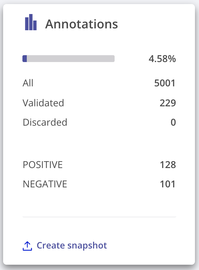
After spending some minutes, we’ve labelled almost 5% of our raw dataset with more than 200 annotated examples, which is a small dataset but should be enough for a first fine-tuning of our banking sentiment classifier:
3. Fine-tune the pre-trained model
In this step, we’ll load our training set from Rubrix and fine-tune using the Trainer API from Hugging Face transformers. For this, we closely follow the guide Fine-tuning a pre-trained model from the transformers docs.

First, let’s load our dataset:
[2]:
rb_df = rb.load(name='labeling_with_pretrained')
This dataset contains all records, let’s filter only our annotations using the status column. The Validated status corresponds to annotated records. You can read more about how record status is defined in Rubrix.
[3]:
rb_df = rb_df[rb_df.status == "Validated"]
[4]:
rb_df.head()
[4]:
| inputs | prediction | annotation | prediction_agent | annotation_agent | multi_label | explanation | id | metadata | status | event_timestamp | |
|---|---|---|---|---|---|---|---|---|---|---|---|
| 4771 | {'text': 'I saw there is a cash withdrawal fro... | [(NEGATIVE, 0.9997006654739381), (POSITIVE, 0.... | [NEGATIVE] | distilbert-base-uncased-finetuned-sst-2-english | .local-Rubrix | False | None | 0001e324-3247-4716-addc-d9d9c83fd8f9 | {'category': 20} | Validated | None |
| 4772 | {'text': 'Why is it showing that my account ha... | [(NEGATIVE, 0.9991878271102901), (POSITIVE, 0.... | [NEGATIVE] | distilbert-base-uncased-finetuned-sst-2-english | .local-Rubrix | False | None | 0017e5c9-c135-44b9-8efb-a17ffecdbe68 | {'category': 34} | Validated | None |
| 4773 | {'text': 'I thought I lost my card but I found... | [(POSITIVE, 0.9842885732650751), (NEGATIVE, 0.... | [POSITIVE] | distilbert-base-uncased-finetuned-sst-2-english | .local-Rubrix | False | None | 0048ccce-8c9f-453d-81b1-a966695e579c | {'category': 13} | Validated | None |
| 4774 | {'text': 'I wanted to top up my account and it... | [(NEGATIVE, 0.999732434749603), (POSITIVE, 0.0... | [NEGATIVE] | distilbert-base-uncased-finetuned-sst-2-english | .local-Rubrix | False | None | 0046aadc-2344-40d2-a930-81f00687bf44 | {'category': 59} | Validated | None |
| 4775 | {'text': 'I need to deposit my virtual card, h... | [(NEGATIVE, 0.9992493987083431), (POSITIVE, 0.... | [POSITIVE] | distilbert-base-uncased-finetuned-sst-2-english | .local-Rubrix | False | None | 00071745-741d-4555-82b3-54d25db44c38 | {'category': 37} | Validated | None |
Prepare training and test datasets
Let’s now prepare our dataset for training and testing our sentiment classifier, using the datasets library:
[ ]:
from datasets import Dataset

# select text input and the annotated label
rb_df['text'] = rb_df.inputs.transform(lambda r: r['text'])
# labels can be a list (for supporting multi-label text classifiers)
# for our problem, we only have one label
rb_df['labels'] = rb_df.annotation.transform(lambda r: r[0])


# create 🤗 dataset from pandas with labels as numeric ids
label2id = {"NEGATIVE": 0, "POSITIVE": 1}
train_ds = Dataset.from_pandas(rb_df[['text', 'labels']])
train_ds = train_ds.map(lambda example: {'labels': label2id[example['labels']]})
[6]:
train_ds = train_ds.train_test_split(test_size=0.2) ; train_ds
[6]:
DatasetDict({
    train: Dataset({
        features: ['__index_level_0__', 'labels', 'text'],
        num_rows: 183
    })
    test: Dataset({
        features: ['__index_level_0__', 'labels', 'text'],
        num_rows: 46
    })
})
[ ]:
from transformers import AutoTokenizer

tokenizer = AutoTokenizer.from_pretrained("distilbert-base-uncased-finetuned-sst-2-english")

def tokenize_function(examples):
    return tokenizer(examples["text"], padding="max_length", truncation=True)

train_dataset = train_ds['train'].map(tokenize_function, batched=True).shuffle(seed=42)
eval_dataset = train_ds['test'].map(tokenize_function, batched=True).shuffle(seed=42)
Train our sentiment classifier
As we mentioned before, we’re going to fine-tune the distilbert-base-uncased-finetuned-sst-2-english model. Another option will be fine-tuning a distilbert masked language model from scratch, we leave this experiment to you.
Let’s load the model:
[1]:
from transformers import AutoModelForSequenceClassification

model = AutoModelForSequenceClassification.from_pretrained("distilbert-base-uncased-finetuned-sst-2-english")
Let’s configure the Trainer:
[ ]:
import numpy as np
from transformers import Trainer
from datasets import load_metric
from transformers import TrainingArguments

training_args = TrainingArguments(
    "distilbert-base-uncased-sentiment-banking",
    evaluation_strategy="epoch",
    logging_steps=30
)

metric = load_metric("accuracy")

def compute_metrics(eval_pred):
    logits, labels = eval_pred
    predictions = np.argmax(logits, axis=-1)
    return metric.compute(predictions=predictions, references=labels)

trainer = Trainer(
    args=training_args,
    model=model,
    train_dataset=train_dataset,
    eval_dataset=eval_dataset,
    compute_metrics=compute_metrics,
)
And finally train our first model!
[ ]:
trainer.train()
4. Testing the fine-tuned model
In this step, let’s first test the model we have just trained.
Let’s create a new pipeline with our model:
[33]:
finetuned_sentiment_classifier = pipeline(
    model=model,
    tokenizer=tokenizer,
    task="sentiment-analysis",
    return_all_scores=True
)
And compare its predictions with the pre-trained model with an example:
[34]:
finetuned_sentiment_classifier(
    'I need to deposit my virtual card, how do i do that.'
), sentiment_classifier(
    'I need to deposit my virtual card, how do i do that.'
)
[34]:
([[{'label': 'NEGATIVE', 'score': 0.0002401248930254951},
   {'label': 'POSITIVE', 'score': 0.9997599124908447}]],
 [[{'label': 'NEGATIVE', 'score': 0.9992493987083435},
   {'label': 'POSITIVE', 'score': 0.0007506058318540454}]])
As you can see, our fine-tuned model now classifies this general questions (not related to issues or problems) as POSITIVE, while the pre-trained model still classifies this as NEGATIVE.
Let’s check now an example related to an issue where both models work as expected:
[35]:
finetuned_sentiment_classifier(
    'Why is my payment still pending?'
), sentiment_classifier(
    'Why is my payment still pending?'
)
[35]:
([[{'label': 'NEGATIVE', 'score': 0.9988037347793579},
   {'label': 'POSITIVE', 'score': 0.001196274533867836}]],
 [[{'label': 'NEGATIVE', 'score': 0.9983781576156616},
   {'label': 'POSITIVE', 'score': 0.0016218466917052865}]])
5. Run our fine-tuned model over the dataset and log the predictions
Let’s now create a dataset from the remaining records (those which we haven’t annotated in the first annotation session).
We’ll do this using the Default status, which means the record hasn’t been assigned a label.
[ ]:
rb_df = rb.load(name='labeling_with_pretrained')
rb_df = rb_df[rb_df.status == "Default"]
rb_df['text'] = rb_df.inputs.transform(lambda r: r['text'])
From here, this is basically the same as step 1, in this case using our fine-tuned model:

[64]:
ds = Dataset.from_pandas(rb_df[['text']])
[65]:
def predict(examples):
    return {"predictions": finetuned_sentiment_classifier(examples['text'])}
[ ]:
ds = ds.map(predict, batched=True, batch_size=8)
[67]:
records = []
for example in ds.shuffle():
    record = rb.TextClassificationRecord(
        inputs=example["text"],
        prediction=[(pred['label'], pred['score']) for pred in example['predictions']],
        prediction_agent="distilbert-base-uncased-banking77-sentiment"
    )
    records.append(record)
[ ]:
rb.log(name='labeling_with_finetuned', records=records)
6. Explore and label data with the fine-tuned model
In this step, we’ll start by exploring how the fine-tuned model is performing with our dataset.
At first sight, using the predicted as filter by POSITIVE and then by NEGATIVE, we see that the fine-tuned model predictions are more aligned with our “annotation policy”.
Now that the model is performing better for our use case, we’ll extend our training set with highly informative examples. A typical workflow for doing this is as follows:
Use the prediction score filter for labeling uncertain examples. Below you can see how to use this filter for labeling examples withing the range from 0 to 0.6.

Label examples predicted as
POSITIVEby our fine-tuned model, and then predicted asNEGATIVEto correct the predictions.
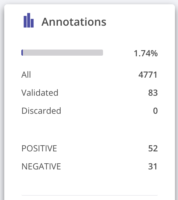
After spending some minutes, we’ve labelled almost 2% of our raw dataset with around 80 annotated examples, which is a small dataset but hopefully with highly informative examples.
7. Fine-tuning with the extended training dataset
In this step, we’ll add the new examples to our training set and fine-tune a new version of our banking sentiment classifier.

Add labeled examples to our previous training set
Let’s add our new examples to our previous training set.
[11]:
def prepare_train_df(dataset_name):
    rb_df = rb.load(name=dataset_name)
    rb_df = rb_df[rb_df.status == "Validated"] ; len(rb_df)
    rb_df['text'] = rb_df.inputs.transform(lambda r: r['text'])
    rb_df['labels'] = rb_df.annotation.transform(lambda r: r[0])
    return rb_df
[12]:
df = prepare_train_df('labeling_with_finetuned') ; len(df)
[12]:
83
[13]:
train_dataset = train_dataset.remove_columns('__index_level_0__')
We’ll use the .add_item method from the datasets library to add our examples:
[14]:
for i,r in df.iterrows():
    tokenization = tokenizer(r["text"], padding="max_length", truncation=True)
    train_dataset = train_dataset.add_item({
        "attention_mask": tokenization["attention_mask"],
        "input_ids": tokenization["input_ids"],
        "labels": label2id[r['labels']],
        "text": r['text'],
    })
[15]:
train_dataset
[15]:
Dataset({
    features: ['attention_mask', 'input_ids', 'labels', 'text'],
    num_rows: 266
})
Train our sentiment classifier
As we want to measure the effect of adding examples to our training set we will:
Fine-tune from the pre-trained sentiment weights (as we did before)
Use the previous test set and the extended train set (obtaining a metric we use to compare this new version with our previous model)
[17]:
from transformers import AutoModelForSequenceClassification
model = AutoModelForSequenceClassification.from_pretrained("distilbert-base-uncased-finetuned-sst-2-english")
[ ]:
train_ds = train_dataset.shuffle(seed=42)

trainer = Trainer(
    args=training_args,
    model=model,
    train_dataset=train_dataset,
    eval_dataset=eval_dataset,
    compute_metrics=compute_metrics,
)

trainer.train()
[ ]:
model.save_pretrained("distilbert-base-uncased-sentiment-banking", push_to_hub=True)
Wrap-up
In this tutorial, you’ve learnt to build a training set from scratch with the help of a pre-trained model, performing two iterations of predict > log > label.
Although this is somehow a toy example, you could apply this workflow to your own projects to adapt existing models or building them from scratch.
In this tutorial, we’ve covered one way of building training sets: hand labeling. If you are interested in other methods, which could be combined witth hand labeling, checkout the following tutorials: