🧱 Extending weak supervision workflows with sentence embeddings#
In this tutorial, we show how weak supervision workflows in Rubrix can be extended with sentence embeddings. We start from the weak supervision workflow presented in our Weak supervision with Rubrix tutorial and improve on its results by extending the coverage of its rules.
✍️ We define rules and generate weak labels for the ag_news data set.
🧱 We extend our weak labels with sentence embeddings from the Sentence Transformers library.
📰 Finally, we use a label model to generate data for training a downstream model as a news classifier.
🚀 We achieve a 4% improvement in accuracy over the original workflow simply by extending our weak labels.
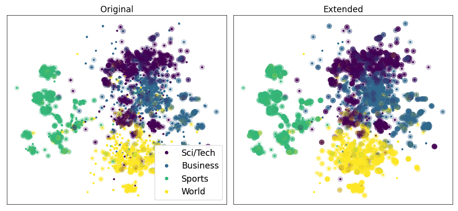
The two plots above show the coverage of the weak labels before and after extending them with embeddings. Each point corresponds to an example in the ag news test set. The color indicates the corresponding class of the example. Points in a transparent circle are covered by at least one rule.
Introduction#
Labelling functions normally have high precision, but low coverage. Only records that strictly match the conditions determined by a given function will be labelled, while other potential candidates will be left out.
Building on the findings of the Hazy Research group, we present a way to solve this problem by extending the weak labels produced by our labelling functions with sentence embeddings.
We extend the coverage of our labelling functions by giving unlabelled records the same label as their nearest labelled neighbor in the embedding space if the cosine similarity between them scores above a certain threshold.
We will show in this tutorial that, by adjusting these similarity thresholds and selecting proper sentence embeddings, we are able to significantly improve the accuracy of the downstream classifiers produced by our weak supervision workflows.
Detailed Workflow#
A typical workflow to perform weak supervision with sentence embeddings is:
Create a Rubrix dataset with your raw dataset. If you have some labelled data, you can log it into the the same dataset.
Define a set of weak labeling rules with the Rules definition mode in the UI.
Create a
WeakLabelsobject and apply the rules. You can load the rules from your dataset and add additional rules and labeling functions using Python. Typically, you’ll iterate between this step and step 2.Extend the
WeakLabelsobject by giving sentence embeddings for each record ( the rows of the matrix ) and a similarity threshold for each rule ( the columns of the matrix ).Once you are satisfied with your extended weak labels, use the extended matrix of the
WeakLabelsinstance with your library/method of choice to build a training set or even train a downstream text classification model. You can iterate between this step and step 4 to try several thresholds and embeddings possibilities until you achieve a satisfactory result.
This guide shows you an end-to-end example using Snorkel. You could alternatively use any other label model available in Rubrix. If you are interested in learning about other options, please check our weak supervision guide.
Setup#
Rubrix, is a free and open-source tool to explore, annotate, and monitor data for NLP projects.
If you are new to Rubrix, check out the ⭐ Github repository.
If you have not installed and launched Rubrix yet, check the Setup and Installation guide.
For this tutorial we also need some third party libraries that can be installed via pip:
[ ]:
%pip install faiss-cpu sentence_transformers transformers datasets
The dataset#
Since this tutorial is an extension of our Weak supervision with Rubrix tutorial, we will also use the ag_news dataset, a well-known benchmark text classification models.
However, to guarantee a fair comparison, we will optimize the thresholds on a validation split, and leave the test split for the final evaluation.
[ ]:
from datasets import load_dataset

agnews = load_dataset("ag_news")

agnews_train, agnews_valid = agnews["train"].train_test_split(test_size=7600, seed=43).values()
1. Create a Rubrix dataset with unlabelled data and test data#
Just like in the first tutorial, let’s load a labelled and unlabelled set of records into Rubrix.
[ ]:
import rubrix as rb

# build our labelled records to evaluate our heuristic rules and optimize the thresholds
records = [
    rb.TextClassificationRecord(
        text=record["text"],
        metadata={"split": "labelled"},
        annotation=agnews_valid.features["label"].int2str(record["label"]),
        id=f"valid_{idx}",
    )
    for idx, record in enumerate(agnews_valid)
]

# build our unlabelled records
records += [
    rb.TextClassificationRecord(
        text=record["text"],
        metadata={"split": "unlabelled"},
        id=f"train_{idx}",
    )
    for idx, record in enumerate(agnews_train)
]

# log the records to Rubrix
rb.log(records, name="news2")
After this step, you have a fully browsable dataset available that you can access via the Rubrix web app.
2. Defining rules#
We will use the same rules as found in the previous tutorial.
[ ]:
from rubrix.labeling.text_classification import Rule

# define queries and patterns for each category (using ES DSL)
queries = [
  (["money", "financ*", "dollar*"], "Business"),
  (["war", "gov*", "minister*", "conflict"], "World"),
  (["footbal*", "sport*", "game", "play*"], "Sports"),
  (["sci*", "techno*", "computer*", "software", "web"], "Sci/Tech")
]

# define rules
rules = [
    Rule(query=term, label=label)
    for terms,label in queries
    for term in terms
]
3. Building and analyzing weak labels#
After building weak labels from our rules, their summary reveals that our rules have, in total, 31% coverage while achieving 74% precision.
[ ]:
from rubrix.labeling.text_classification import WeakLabels

# apply the rules to the dataset to obtain the weak labels
weak_labels = WeakLabels(
    rules=rules,
    dataset="news2"
)
[5]:
weak_labels.summary()
[5]:
| label | coverage | annotated_coverage | overlaps | conflicts | correct | incorrect | precision | |
|---|---|---|---|---|---|---|---|---|
| money | {Business} | 0.008242 | 0.008816 | 0.002450 | 0.001925 | 31 | 36 | 0.462687 |
| financ* | {Business} | 0.019775 | 0.021184 | 0.005892 | 0.005183 | 115 | 46 | 0.714286 |
| dollar* | {Business} | 0.016608 | 0.016974 | 0.003492 | 0.002850 | 98 | 31 | 0.759690 |
| war | {World} | 0.011683 | 0.008816 | 0.003242 | 0.001367 | 44 | 23 | 0.656716 |
| gov* | {World} | 0.045067 | 0.043158 | 0.010800 | 0.006225 | 156 | 172 | 0.475610 |
| minister* | {World} | 0.030142 | 0.030263 | 0.007508 | 0.002825 | 207 | 23 | 0.900000 |
| conflict | {World} | 0.003050 | 0.003684 | 0.001025 | 0.000092 | 20 | 8 | 0.714286 |
| footbal* | {Sports} | 0.013050 | 0.015132 | 0.004875 | 0.000408 | 105 | 10 | 0.913043 |
| sport* | {Sports} | 0.021183 | 0.021711 | 0.007033 | 0.001225 | 146 | 19 | 0.884848 |
| game | {Sports} | 0.038950 | 0.043026 | 0.014067 | 0.002375 | 253 | 74 | 0.773700 |
| play* | {Sports} | 0.052608 | 0.057632 | 0.016767 | 0.004992 | 312 | 126 | 0.712329 |
| sci* | {Sci/Tech} | 0.016433 | 0.015658 | 0.002742 | 0.001275 | 101 | 18 | 0.848739 |
| techno* | {Sci/Tech} | 0.027150 | 0.028816 | 0.008325 | 0.003108 | 153 | 66 | 0.698630 |
| computer* | {Sci/Tech} | 0.027275 | 0.026447 | 0.011100 | 0.004483 | 167 | 34 | 0.830846 |
| software | {Sci/Tech} | 0.030283 | 0.032763 | 0.009625 | 0.003308 | 202 | 47 | 0.811245 |
| web | {Sci/Tech} | 0.015508 | 0.016316 | 0.004100 | 0.001608 | 111 | 13 | 0.895161 |
| total | {Sci/Tech, World, Sports, Business} | 0.317375 | 0.327895 | 0.053408 | 0.019425 | 2221 | 746 | 0.748568 |
In the next steps, we will try to extend our weak labels matrix through sentence embeddings. In this way, we will increase the coverage of our rules, while maintaining an acceptable precision.
4. Using the weak labels#
Label model with Snorkel#
Snorkel’s label model is by far the most popular option for using weak supervision, and Rubrix provides built-in support for it. Here we fit our weak labels to the Snorkel label model, and then we check the performance on the records that have been covered by the rules.
[6]:
from rubrix.labeling.text_classification import Snorkel

# create the the Snorkel label model
label_model = Snorkel(weak_labels)

# fit the model, for the learning rate and epochs we ran a quick grid search
label_model.fit(lr=0.002, n_epochs=10, progress_bar=False)

# evaluate the label model
print(label_model.score(output_str=True))
              precision    recall  f1-score   support

    Business       0.73      0.41      0.53       493
      Sports       0.77      0.97      0.86       703
       World       0.69      0.83      0.75       462
    Sci/Tech       0.80      0.74      0.77       833

    accuracy                           0.76      2491
   macro avg       0.75      0.74      0.73      2491
weighted avg       0.76      0.76      0.74      2491
5. Extending the weak labels#
Let’s extend our weak labels and see how that impacts the evaluation of the Snorkel label model.
Generate sentence embeddings#
Let’s generate sentence embeddings for each record of our weak labels matrix. Best results will be achieved through powerful general-purpose pretrained embeddings, or by embeddings especifically pretrained for the domain of the task at hand.
Here we choose the all-mpnet-base-v2 embeddings from the well-known Sentence Transformers library. Rubrix allows us to experiment with embeddings from any source, as long as they are provided to the weak labels matrix as a two-dimensional array.
For instance, instead of Sentence Transformers, we could have utilized GPT-3 similarity embeddings from the OpenAI Embeddings API, or text embeddings from the Tensorflow Hub, or we could even have trained our own embeddings from scratch.
[ ]:
from sentence_transformers import SentenceTransformer
from tqdm.auto import tqdm

# instantiate the model for the sentence embeddings
# we strongly recommend using a GPU for the computation of the embeddings
model = SentenceTransformer('all-mpnet-base-v2', device='cuda')

# compute the embeddings and store them in a list
embeddings = []
for rec in tqdm(weak_labels.records()):
    embeddings.append(model.encode(rec.text))
Set the thresholds#
We start by making an educated guess on which thresholds will work for this particular weak labels matrix. We set the thresholds for all rules to 0.60. This means that, for each rule, the label of a record will be extended to its nearest unlabelled neighbor if their cosine similarity is above this value.
[ ]:
thresholds = [0.6] * len(rules)
Extend the weak labels matrix#
We call the extend_matrix method by providing the thresholds and the sentence embeddings.
[ ]:
weak_labels.extend_matrix(thresholds, embeddings)
With the weak label matrix extended, we can check that our coverage went up significantly (from 0.32 to 0.79).
[10]:
weak_labels.summary()
[10]:
| label | coverage | annotated_coverage | overlaps | conflicts | correct | incorrect | precision | |
|---|---|---|---|---|---|---|---|---|
| money | {Business} | 0.079342 | 0.083158 | 0.068042 | 0.061908 | 342 | 290 | 0.541139 |
| financ* | {Business} | 0.122692 | 0.130526 | 0.096475 | 0.087525 | 596 | 396 | 0.600806 |
| dollar* | {Business} | 0.104917 | 0.110789 | 0.084467 | 0.077458 | 552 | 290 | 0.655582 |
| war | {World} | 0.083958 | 0.081053 | 0.069425 | 0.050867 | 353 | 263 | 0.573052 |
| gov* | {World} | 0.218817 | 0.216447 | 0.157083 | 0.118283 | 843 | 802 | 0.512462 |
| minister* | {World} | 0.124367 | 0.121974 | 0.091817 | 0.055133 | 752 | 175 | 0.811219 |
| conflict | {World} | 0.038975 | 0.036579 | 0.035533 | 0.023192 | 199 | 79 | 0.715827 |
| footbal* | {Sports} | 0.040083 | 0.043289 | 0.029475 | 0.007708 | 308 | 21 | 0.936170 |
| sport* | {Sports} | 0.114292 | 0.111053 | 0.084200 | 0.031992 | 745 | 99 | 0.882701 |
| game | {Sports} | 0.125608 | 0.130526 | 0.094600 | 0.035858 | 745 | 247 | 0.751008 |
| play* | {Sports} | 0.205158 | 0.206053 | 0.156583 | 0.091692 | 900 | 666 | 0.574713 |
| sci* | {Sci/Tech} | 0.058375 | 0.056053 | 0.035192 | 0.028675 | 257 | 169 | 0.603286 |
| techno* | {Sci/Tech} | 0.117850 | 0.124079 | 0.092108 | 0.074517 | 558 | 385 | 0.591729 |
| computer* | {Sci/Tech} | 0.100017 | 0.097632 | 0.079608 | 0.060317 | 553 | 189 | 0.745283 |
| software | {Sci/Tech} | 0.088967 | 0.088816 | 0.065025 | 0.046550 | 517 | 158 | 0.765926 |
| web | {Sci/Tech} | 0.084800 | 0.081579 | 0.067950 | 0.054550 | 415 | 205 | 0.669355 |
| total | {Sci/Tech, Sports, Business, World} | 0.793542 | 0.793553 | 0.392908 | 0.228892 | 8635 | 4434 | 0.660724 |
We also see that the average precision of our rules went down (from 0.75 to 0.66). This drop, however, can be partially compensated by our label model. If we fit our weak labels to a Snorkel label model again, we can see that the support went up significantly, as expected, while the drop in accuracy is minor.
[12]:
label_model = Snorkel(weak_labels)
label_model.fit(lr=0.002, n_epochs=10, progress_bar=False)
print(label_model.score(output_str=True))
              precision    recall  f1-score   support

    Sci/Tech       0.76      0.74      0.75      1636
       World       0.67      0.86      0.76      1421
      Sports       0.79      0.96      0.87      1544
    Business       0.78      0.39      0.52      1430

    accuracy                           0.74      6031
   macro avg       0.75      0.74      0.72      6031
weighted avg       0.75      0.74      0.73      6031
You can have a look at the Appendix to have a detailed explanation about how the weak label matrix is extended under the hood.
Instead of using generic fixed thresholds, we recommend to optimize them in some way to get the highest performance gains. Our optimization described in detail in the Appendix yielded following thresholds:
[ ]:
optimized_thresholds = [0.4, 0.4, 0.6, 0.4, 0.5, 0.8, 1., 0.4, 0.4, 0.5, 0.6, 0.4, 0.4, 0.6, 0.6, 0.8]
Each call to extend_matrix with thresholds and embeddings will build a faiss index that will be cached inside the weak labels object.
If we do not provide embeddings in our next calls to extend_matrix, this index will be reutilized, and a new extended matrix will replace the current extended matrix. So extending the matrix with new threshold is very cheap.
[28]:
weak_labels.extend_matrix(optimized_thresholds)
label_model = Snorkel(weak_labels)
label_model.fit(lr=0.002, n_epochs=10, progress_bar=False)
print(label_model.score(output_str=True))
              precision    recall  f1-score   support

    Sci/Tech       0.74      0.67      0.70      1906
       World       0.78      0.64      0.70      1789
      Sports       0.82      0.90      0.86      1875
    Business       0.60      0.69      0.64      1877

    accuracy                           0.73      7447
   macro avg       0.73      0.73      0.73      7447
weighted avg       0.73      0.73      0.73      7447
The optimized thresholds seem to further reduce the accuracy of the label model, but also increase the coverage significantly.
6. Training a downstream model#
Now we will train the same dowstream model as in the previous tutorial, but on the data produced by a label model from our extended weak labels.
Let us first define a helper function that is basically a copy&paste from the previous tutorial.
[ ]:
import pandas as pd
from sklearn.feature_extraction.text import CountVectorizer
from sklearn.naive_bayes import MultinomialNB
from sklearn.pipeline import Pipeline
from sklearn import metrics


def train_and_evaluate_downstream_model(label_model):
    """
    Train a downstream model with the predictions of a label model and
    evauate it with the test split of the ag news dataset
    """
    # get records with the predictions from the label model
    records = label_model.predict()

    # turn str labels into integers
    label2int = label_model.weak_labels.label2int

    # extract training data
    X_train = [rec.text for rec in records]
    y_train = [label2int[rec.prediction[0][0]] for rec in records]

    # define our final classifier
    classifier = Pipeline([
        ('vect', CountVectorizer()),
        ('clf', MultinomialNB())
    ])

    # fit the classifier
    classifier.fit(
        X=X_train,
        y=y_train,
    )

    # extract text and labels
    X_test = [rec["text"] for rec in agnews["test"]]
    y_test = [label2int[agnews["test"].features["label"].int2str(rec["label"])] for rec in agnews["test"]]

    # get predictions for the test set
    predicted = classifier.predict(X_test)

    return metrics.classification_report(y_test, predicted, target_names=[k for k in label2int.keys() if k])
Now let’s see how our downstream model compares with the original model from the previous tutorial. Remember we achieved an accuracy of around 82%.
[35]:
print(train_and_evaluate_downstream_model(label_model))
              precision    recall  f1-score   support

    Sci/Tech       0.85      0.82      0.83      1900
       World       0.90      0.84      0.87      1900
      Sports       0.90      0.97      0.93      1900
    Business       0.81      0.82      0.81      1900

    accuracy                           0.86      7600
   macro avg       0.86      0.86      0.86      7600
weighted avg       0.86      0.86      0.86      7600
Now, with our extended weak label matrix, we were able to achieve an accuracy of 86%, a 4% improvement over our original approach.
Summary#
In this tutorial you have seen how to improve your weak supervision workflows in Rubrix using word embeddings. With very small changes to the original workflow, we were able to significantly increase the accuracy of our downstream models. This shows that Rubrix can greatly reduce the amount of effort that human annotators need to put into writing rules before they can achieve exceptional results.
Next steps#
⭐ Rubrix Github repo to stay updated.
📚 Rubrix documentation for more guides and tutorials.
🙋♀️ Join the Rubrix community! A good place to start is the discussion forum.
Appendix: Visualize changes#
Let’s visualize how the weak labels matrix is being extended in a single row.
[ ]:
import pandas as pd

def get_transitions(weak_labels, idx):
    transitions = list(list(zip(row[0], row[1])) for row in zip(weak_labels._matrix, weak_labels._extended_matrix))
    transitions = transitions[idx]
    label_dict = weak_labels.int2label
    rule_labels = weak_labels.summary().reset_index()['index'].values.tolist()[:-1]
    transitions_df = []
    for rule_idx, rule in enumerate(rule_labels):
        old_label = transitions[rule_idx][0]
        new_label = transitions[rule_idx][1]
        transitions_df.append({
            "rule": rule,
            "old label": label_dict[old_label],
            "new label": label_dict[new_label],
        })
    transitions_df = pd.DataFrame(transitions_df)
    text = weak_labels.records()[idx].text
    return transitions_df, text

transitions, text = get_transitions(weak_labels, 15)
By reading the selected record, we can clearly notice that it is a news article about world politics, and therefore should be classified as World.
[79]:
text
[79]:
'Israel #39;determined to complete Gaza plan #39; Israel is determined to go ahead with its unilateral withdrawal from the Gaza Strip - regardless of the death of Yasser Arafat and even if settlers resist - a top Israeli general who helped design the plan says.'
Let’s put side by side the row of the original weak labels matrix for this record ( the "old label" row ) and the same row after extension ( the "new label" row ).
We see that this news article was not labelled in the original matrix by any of our rules.
However, it was the nearest unlabelled neighbor of two Business articles, matched by the rules financ* and dollar*, and its similarity with them scored above our selected thresholds. The same happened for two World articles, matched by the rules war and minister*, and for a Sci/Tech article matched by the rule sci*.
[80]:
transitions.transpose()
[80]:
| 0 | 1 | 2 | 3 | 4 | 5 | 6 | 7 | 8 | 9 | 10 | 11 | 12 | 13 | 14 | 15 | |
|---|---|---|---|---|---|---|---|---|---|---|---|---|---|---|---|---|
| rule | money | financ* | dollar* | war | gov* | minister* | conflict | footbal* | sport* | game | play* | sci* | techno* | computer* | software | web |
| old label | None | None | None | None | None | None | None | None | None | None | None | None | None | None | None | None |
| new label | None | Business | Business | World | None | World | None | None | None | None | None | Sci/Tech | None | None | None | None |
Appendix: Optimizing the thresholds#
Each call to extend_matrix with thresholds and embeddings will build a faiss index that will be cached inside the weak labels object.
If we do not provide embeddings in our next calls to extend_matrix, this index will be reutilized, and a new extended matrix will replace the current extended matrix. This new matrix is an extension of the original weak labels matrix made according to our new similarity thresholds.
[ ]:
# Let's try to set all thresholds to 0.8 instead of 0.6.
thresholds = [0.8] * len(rules)

# As we have already generated the index in our first call, we just need to provide the thresholds.
weak_labels.extend_matrix(thresholds)
There are a few different approaches to find the best similarity thresholds for extending a weak labels matrix: we will list them from the least to the most computationally expensive.
1. Block the extension of low overlap rules#
After setting all similarity thresholds to a reasonable value, a good way to optimize the similarity thresholds on an individual level is to block the extension of rules with low overlap, as they are more likely to produce inaccurate results after extension.
[111]:
summary = weak_labels.summary(normalize_by_coverage=True).reset_index().head(len(rules))
summary = summary.rename(columns={"index":"rule"})
summary = summary.sort_values(by="overlaps", ascending=True)[["rule", "overlaps"]]
summary = summary.reset_index()
summary
[111]:
| index | rule | overlaps | |
|---|---|---|---|
| 0 | 4 | gov* | 0.239645 |
| 1 | 15 | web | 0.264374 |
| 2 | 14 | software | 0.317832 |
| 3 | 10 | play* | 0.318707 |
| 4 | 6 | conflict | 0.336066 |
| 5 | 9 | game | 0.361147 |
| 6 | 8 | sport* | 0.393875 |
| 7 | 11 | sci* | 0.483512 |
| 8 | 5 | minister* | 0.514205 |
| 9 | 7 | footbal* | 0.567152 |
| 10 | 13 | computer* | 0.703716 |
| 11 | 12 | techno* | 0.710083 |
| 12 | 1 | financ* | 0.737078 |
| 13 | 2 | dollar* | 0.742097 |
| 14 | 3 | war | 0.744417 |
| 15 | 0 | money | 0.788047 |
[112]:
thresholds = [0.6] * len(rules)

# Let's block the extension of the top 5 rules with the least overlap.
turn_off_index = summary['index'][0:6]

# We block the extension of a rule by setting its similarity threshold to 1.0.
for rule_index in turn_off_index:
    thresholds[rule_index] = 1.0

weak_labels.extend_matrix(thresholds)
label_model = Snorkel(weak_labels)
label_model.fit(lr=0.002, n_epochs=10, progress_bar=False)
print(train_and_evaluate_downstream_model(label_model))
              precision    recall  f1-score   support

    Sci/Tech       0.81      0.84      0.82      1900
       World       0.90      0.87      0.88      1900
      Sports       0.91      0.96      0.93      1900
    Business       0.81      0.76      0.78      1900

    accuracy                           0.86      7600
   macro avg       0.85      0.86      0.85      7600
weighted avg       0.85      0.86      0.85      7600
2. Brute force: Grid search over the label model#
In this approach, we set all thresholds to an initial value, and then grid search for the best value for each one of them individually. Then we optimize for the harmonic mean between the coverage and the accuracy of the label model on the development set. This will ensure that we choose the thresholds with the best trade-off between both metrics.
We arrive at the same improvement as the previous approach, with a final accuracy of 86% over the test set.
[ ]:
def train_eval_labelmodel(ths):
    weak_labels.extend_matrix(ths)

    label_model = Snorkel(weak_labels)
    label_model.fit(lr=0.002, n_epochs=10, progress_bar=False)

    metrics = label_model.score()
    acc, sup, n = metrics["accuracy"], metrics["macro avg"]["support"], len(weak_labels.annotation())
    coverage = sup / n
    return 2 * acc * coverage / ( acc + coverage )
[ ]:
import copy
from tqdm.auto import tqdm

ths_range = np.arange(1, 0.3, -0.1)
n_ths = len(weak_labels.rules)

best_thresholds = [1.0] * n_ths
best_acc = 0.0
for i in tqdm(range(n_ths), total=n_ths):
    thresholds = best_thresholds.copy()
    for threshold in ths_range:
        thresholds[i] = threshold
        acc = train_eval_labelmodel(thresholds)
        if acc > best_acc:
            best_acc = acc
            best_thresholds = thresholds.copy()
[121]:
np.array(best_thresholds)
[121]:
array([0.4, 0.4, 0.6, 0.4, 0.5, 0.8, 1. , 0.4, 0.4, 0.5, 0.6, 0.4, 0.4,
       0.6, 0.6, 0.8])
[122]:
weak_labels.extend_matrix(best_thresholds)
label_model = Snorkel(weak_labels)
label_model.fit(lr=0.002, n_epochs=10, progress_bar=False)
print(train_and_evaluate_downstream_model(label_model))
              precision    recall  f1-score   support

    Sci/Tech       0.83      0.83      0.83      1900
       World       0.89      0.85      0.87      1900
      Sports       0.90      0.97      0.93      1900
    Business       0.82      0.79      0.80      1900

    accuracy                           0.86      7600
   macro avg       0.86      0.86      0.86      7600
weighted avg       0.86      0.86      0.86      7600
3. Brute force: Grid search over the downstream model#
Here again we set all thresholds to an initial value and grid search for the best value for each individual threshold, but now we optimize for the accuracy of the downstream model on the development set. We arrive at a final accuracy of 85% on the test set, which is slightly less than what we achieved through the previous approaches.
[126]:
# retrieve records with annotations
test_ds = weak_labels.records(has_annotation=True)

# extract text and labels
X_test_for_grid_search = [rec.text for rec in test_ds]
y_test_for_grid_search = [weak_labels.label2int[rec.annotation] for rec in test_ds]

def train_eval_downstream(ths):
    weak_labels.extend_matrix(ths)

    label_model = Snorkel(weak_labels)
    label_model.fit(lr=0.002, n_epochs=10, progress_bar=False)

    records = label_model.predict()

    X_train = [rec.text for rec in records]
    y_train = [weak_labels.label2int[rec.prediction[0][0]] for rec in records]

    classifier = Pipeline([
        ('vect', CountVectorizer()),
        ('clf', MultinomialNB())
    ])

    classifier.fit(
        X=X_train,
        y=y_train,
    )

    accuracy = classifier.score(
        X=X_test_for_grid_search,
        y=y_test_for_grid_search,
    )

    return accuracy
[ ]:
from copy import copy
from tqdm.auto import tqdm

best_thresholds, best_acc = [1.0] * len(weak_labels.rules), 0
ths_range = np.arange(1, 0.3, -0.1)
n_ths = len(weak_labels.rules)

for i in tqdm(range(n_ths), total=n_ths):
    thresholds = best_thresholds.copy()
    for threshold in ths_range:
        thresholds[i] = threshold
        acc = train_eval_downstream(thresholds)
        if acc > best_acc:
            best_acc = acc
            best_thresholds = thresholds.copy()
[128]:
np.array(best_thresholds)
[128]:
array([0.6, 0.7, 0.9, 1. , 1. , 0.8, 0.7, 1. , 0.6, 1. , 1. , 0.7, 0.8,
       0.7, 0.9, 0.8])
[129]:
weak_labels.extend_matrix(best_thresholds)
label_model = Snorkel(weak_labels)
label_model.fit(lr=0.002, n_epochs=10, progress_bar=False)
print(train_and_evaluate_downstream_model(label_model))
              precision    recall  f1-score   support

    Sci/Tech       0.81      0.82      0.82      1900
       World       0.89      0.85      0.87      1900
      Sports       0.88      0.98      0.93      1900
    Business       0.82      0.75      0.78      1900

    accuracy                           0.85      7600
   macro avg       0.85      0.85      0.85      7600
weighted avg       0.85      0.85      0.85      7600
Tips on threshold optimization#
Grid search with large downstream models, such as transformers, can be very expensive. In this scenario, we can consider to optimize only a subset of the thresholds, or to optimize all thresholds on a small sample of the development set.
Although in this tutorial we perform grid search sequentially, there is no impediment to speed it up by performing it in parallel, as long as we make deep copies of the weak labels object for each process or thread.
Appendix: Plot extension#
[ ]:
import umap
import matplotlib.pyplot as plt

umap_data = umap.UMAP(n_neighbors=15, n_components=2, min_dist=0.0, metric='cosine').fit_transform(embeddings)

df = rb.DatasetForTextClassification(weak_labels.records()).to_pandas()
df["x"], df["y"] = umap_data[:, 0], umap_data[:, 1]
df["wl"] = [em for em in weak_labels._matrix]
df["wl_ext"] = [em for em in weak_labels._extended_matrix]

cov_idx = df["wl"].map(lambda x: x.sum() != -16)
cov_ext_idx = df["wl_ext"].map(lambda x: x.sum() != -16)
test_idx = ~(df.annotation.isna())

df_test = df[test_idx]
df_cov, df_cov_ext = df[cov_idx & test_idx], df[cov_ext_idx & test_idx]

label2int = {label: i for i, label in enumerate(df_test.annotation.value_counts().index)}

fig, ax = plt.subplots(1, 2, figsize=(13, 6), )

ax[0].scatter(df_test.x, df_test.y, c=df_test.annotation.map(lambda x: label2int[x]), s=10)
ax[0].scatter(df_cov.x, df_cov.y, c=df_cov.annotation.map(lambda x: label2int[x]), s=100, alpha=0.2)

scatter = ax[1].scatter(df_test.x, df_test.y, c=df_test.annotation.map(lambda x: label2int[x]), s=10)
ax[1].scatter(df_cov_ext.x, df_cov_ext.y, c=df_cov_ext.annotation.map(lambda x: label2int[x]), s=100, alpha=0.2)

ax[0].set_title("Original",{"fontsize": "xx-large"})
ax[0].set_xticks([]), ax[0].set_yticks([])

ax[1].set_title("Extended",{"fontsize": "xx-large"})
ax[1].set_xticks([]), ax[1].set_yticks([])

labels = list(scatter.legend_elements())
labels[1] = list(label2int.keys())
legend1 = ax[0].legend(*labels, loc="lower right", fontsize="xx-large")
ax[0].add_artist(legend1)

fig.tight_layout()
plt.savefig("extend_weak_labels.png", facecolor='white', transparent=False)